Running the executables

Running ARES: basic run on 2M++

Introduction

First of course please build ARES. We will call $BUILD, the directory where you built the entire code. By default it is located in the source directory in the subdirectory build. But if you have specified a different directory with the argument “–build-dir”, then $BUILD represent that last directory name. We will also call $SOURCE the top source directory of ARES. In that case $SOURCE/README.rst would point to the README file at the top source directory.

After a successful build you should find a binary program in $BUILD/src/ares3. This is the main ARES3 program. If you type $BUILD/src/ares3, then you should get the following output:

setupMPI with threads
Initializing console.
[0/1] [DEBUG  ] INIT: MPI/FFTW
[STD    ]
[STD    ]        o
[STD    ]     ,-.|____________________
[STD    ]  O==+-|(>-------- --  -     .>
[STD    ]     `- |"""""""d88b"""""""""
[STD    ]      | o     d8P 88b
[STD    ]      |  \    98=, =88
[STD    ]      |   \   8b _, 88b
[STD    ]      `._ `.   8`..'888
[STD    ]       |    \--'\   `-8___        __________________________________
[STD    ]       \`-.              \                        ARES3
[STD    ]         `. \ -       - / <          (c) Jens Jasche 2012 - 2017
[STD    ]           \ `---   ___/|_-\             Guilhem Lavaux 2014 - 2017
[STD    ]            |._      _. |_-|      __________________________________
[STD    ]            \  _     _  /.-\
[STD    ]             | -! . !- ||   |
[STD    ]             \ "| ^ |" /\   |
[STD    ]             =oO)<>(Oo=  \  /
[STD    ]              d8888888b   < \
[STD    ]             d888888888b  \_/
[STD    ]             d888888888b
[STD    ]
[STD    ] Please acknowledge XXXX
[0/1] [DEBUG  ] INIT: FFTW/WISDOM
[0/1] [INFO   ] Starting ARES3. rank=0, size=1
[0/1] [INFO   ] ARES3 base version c9e74ec93121f9d99a3b2fecb859206b4a8b74a3
[0/1] [ERROR  ] ARES3 requires exactly two parameters: INIT or RESUME as first parameter and the configuration file as second parameter.

We will now go step by step for this output:

First we encounter setupMPI with threads, it means the code asks for the MPI system to support multithreading for hybrid parallelization. The console is then initialized as it needs MPI to properly chose which file should receive the output.
After that the console logs get a prefix [R/N], with R and N integers. R is the MPI rank of the task emitting the information, and N is total number of MPI tasks. Then there is another [ XXXX ], where XXXX indicates the console log level. The amount of output you get is dependent on some flags in the configuration file. But by default you get everything, till the ini file is read. Note that “STD” level is only printed on the task of rank 0.
Then [0/1] [DEBUG ] INIT: MPI/FFTW indicates that the code asks for the MPI variant of FFTW to be initialized. It means the code is indeed compiled with FFTW with MPI support.
The ascii art logo is then shown.
[0/1] [DEBUG ] INIT: FFTW/WISDOM indicates the wisdom is attempted to be recovered for faster FFTW plan constructions.
[0/1] [INFO ] Starting ARES3. rank=0, size=1 Reminds you that we are indeed starting an MPI run.
ARES3 base version XXXX gives the git version of the ARES base git repository used to construct the binary. In case of issue it is nice to report this number to check if any patch has been applied compared to other repository and make debugging life easier.
Finally you get an error:
```
ARES3 requires exactly two parameters: INIT or RESUME as first parameter and the configuration file as second parameter,
```
which tells you that you need to pass down two arguments: the first one is either “INIT” or “RESUME” (though more flags are available but they are documented later on) and the second is the parameter file.

First run

Now we can proceed with setting up an actual run. You can use the files available in $SOURCE/examples/. There are (as of 27.10.2020) ini files for running the executables on the given datasets (in this case the 2MPP dataset). Create a directory (e.g. test_ares/, which we call $TEST_DIR) and now proceeds as follow:

cd $TEST_DIR
$BUILD/src/ares3 INIT $SOURCE/examples/2mpp_ares3.ini

Note if you are using SLURM, you should execute with srun. With the above options ares3 will start as a single MPI task, and allocate as many parallel threads as the computer can support. The top of the output is the following (after the splash and the other outputs aforementioned):

[0/1] [DEBUG  ] Parsing ini file
[0/1] [DEBUG  ] Retrieving system tree
[0/1] [DEBUG  ] Retrieving run tree
[0/1] [DEBUG  ] Creating array which is UNALIGNED
[0/1] [DEBUG  ] Creating array which is UNALIGNED
[INFO S ] Got base resolution at 64 x 64 x 64
[INFO S ] Data and model will use the folllowing method: 'Nearest Grid point number count'
[0/1] [INFO   ] Initializing 4 threaded random number generators
[0/1] [INFO   ] Entering initForegrounds
[0/1] [INFO   ] Done
[INFO S ] Entering loadGalaxySurveyCatalog(0)
[STD    ] | Reading galaxy survey file '2MPP.txt'
[0/1] [WARNING] | I used a default weight of 1
[0/1] [WARNING] | I used a default weight of 1
[STD    ] | Receive 67224 galaxies in total
[INFO S ] | Set the bias to [1]
[INFO S ] | No initial mean density value set, use nmean=1
[INFO S ] | Load sky completeness map 'completeness_11_5.fits.gz'

Again, we will explain some of these lines

Got base resolution at 64 x 64 x 64 indicates ARES understands you want to use a base grid of 64x64x64. In the case of HADES however multiple of this grid may be used.
Data and model will use the folllowing method: 'Nearest Grid point number count' indicates that galaxies are going to binned.
[0/1] [INFO ] Initializing 4 threaded random number generators, we clearly see here that the code is setting up itself to use 4 threads. In particular the random number generator is getting seeded appropriately to generate different sequences on each of the thread.
[STD ] | Reading galaxy survey file '2MPP.txt' indicates the data are being read from the indicated file.
[0/1] [WARNING] | I used a default weight of 1, in the case of this file there is a missing last column which can indicate the weight. By default it gets set to one.

The code then continues proceeding. All the detailed outputs are sent to logares.txt_rank_0 . The last digit indices the MPI rank task , as each task will output in its own file to avoid synchronization problems. Also it reduces the clutter in the final file.

Restarting

If for some reason you have to interrupt the run, then it is not a problem to resuming it at the same place. ARES by default saves a restart file each time a MCMC file is emitted. This can be reduced by changing the flag “savePeriodicity” to an integer number indicating the periodicity (i.e. 5 to emit a restart file every 5 mcmc files).

Then you can resume the run using: $BUILD/src/ares3 RESUME 2mpp.ini. ARES will initialize itself, then reset its internal state using the values contained in the restart file. Note that there is one restart file per MPI task (thus the suffix _0 if you are running with only the multithreaded mode).

Checking the output

After some (maybe very long) time, you can check the output files that have been created by ARES. By default the ini file is set to run for 10,000 samples, so waiting for the end of the run will take possibly several hours on a classic workstation. The end of the run will conclude like:

[STD    ] Reached end of the loop. Writing restart file.
[0/1] [INFO   ] Cleaning up parallel random number generators
[0/1] [INFO   ] Cleaning up Messenger-Signal
[0/1] [INFO   ] Cleaning up Powerspectrum sampler (b)
[0/1] [INFO   ] Cleaning up Powerspectrum sampler (a)

Looking at the powerspectrum

Now we are going to set the PYTHONPATH to $SOURCE/scripts. I.e., if you are using bash you can run the following piece:

PYTHONPATH=$SOURCE/scripts:$PYTHONPATH
export PYTHONPATH

Then we can start analyzing the powerspectrum of the elements of the chain. You can copy paste the following code in a python file (let’s call it show_powerspectrum.py) and run it with your python3 interpreter (depending on your installation it can be python3, python3.5, python3.6 or later):

import matplotlib
matplotlib.use('Agg')
import matplotlib.pyplot as plt
import ares_tools as at

chain = at.read_chain_h5(".", ['scalars.powerspectrum'])

meta = at.read_all_h5("restart.h5_0", lazy=True)

fig = plt.figure(1)
ax = fig.add_subplot(111)
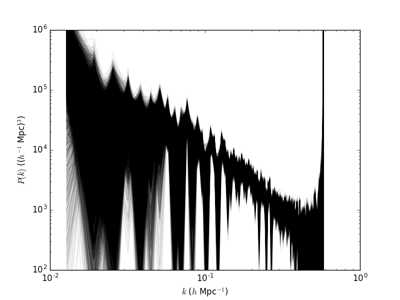
ax.loglog(meta.scalars.k_modes, chain['scalars.powerspectrum'].transpose(),color='k',alpha=0.05)
ax.set_xlim(1e-2,1)
ax.set_ylim(1e2,1e6)
ax.set_xlabel('$k$ ($h$ Mpc$^{-1}$)')
ax.set_ylabel('$P(k)$ (($h^{-1}$ Mpc)$^3$)')

fig.savefig("powerspectrum.png")

We will see what each of the most important lines are doing:

line 1-2: we import matplotlib and enforce that we only need the Agg backend (to avoid needing a real display connection).
line 4: we import the ares_tools analysis scripts
line 6: we ask to read the entire chain contained in the current path ("."). Also we request to obtain the field scalars.powerspectrum from each file. The result is stored in a named column array chain. We could have asked to only partially read the chain using the keyword start, end or step. Some help is available using the command help(at.read_chain_h5).
line 8: we ask to read the entirety of restart.h5_0, however it is done lazily (lazy=True), meaning the data is not read in central memory but only referenced to data in the file. The fields of the file are available as recursive objects in meta. For example, scalars.k_modes here is available as the array stored as meta.scalars.k_modes. While we are at looking this array, it corresponds to the left side of the bins of powerspectra contained in scalars.powerspectrum.
line 12: we plot all the spectra using k_modes on the x-axis and the content of chain['scalars.powerspectrum'] on the y-axis. The array is transposed so that we get bins in k on the first axis of the array, and each sample on the second one. This allows to use only one call to ax.loglog.
line 18: we save the result in the given image file.

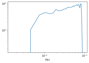
After this script is run, you will get a plot containing all the sampled powerspectra in the chain. It is saved in powerspectrum.png

Running this script will result typically in the following plot (here for 10,000 samples):

running/ARES_Tutorials_files/Powerspectrum_tutorial1_ares.png

Looking at the density field

Now we can also compute the aposteriori mean and standard deviation per voxel of the matter density field. The following script does exactly this:

import matplotlib
matplotlib.use('Agg')
import matplotlib.pyplot as plt
import numpy as np
import ares_tools as at

density = at.read_chain_avg_dev(".", ['scalars.s_field'], slicer=lambda x: x[32,:,:], do_dev=True, step=1)

meta = at.read_all_h5("restart.h5_0", lazy=True)

L = meta.scalars.L0[0]
N = meta.scalars.N0[0]

ix = np.arange(N)*L/(N-1) - 0.5*L

fig = plt.figure(1, figsize=(16,5))
ax = fig.add_subplot(121)
im = ax.pcolormesh(ix[:,None].repeat(N,axis=1), ix[None,:].repeat(N,axis=0), density['scalars.s_field'][0],vmin=-1,vmax=2)
ax.set_aspect('equal')
ax.set_xlim(-L/2,L/2)
ax.set_ylim(-L/2,L/2)
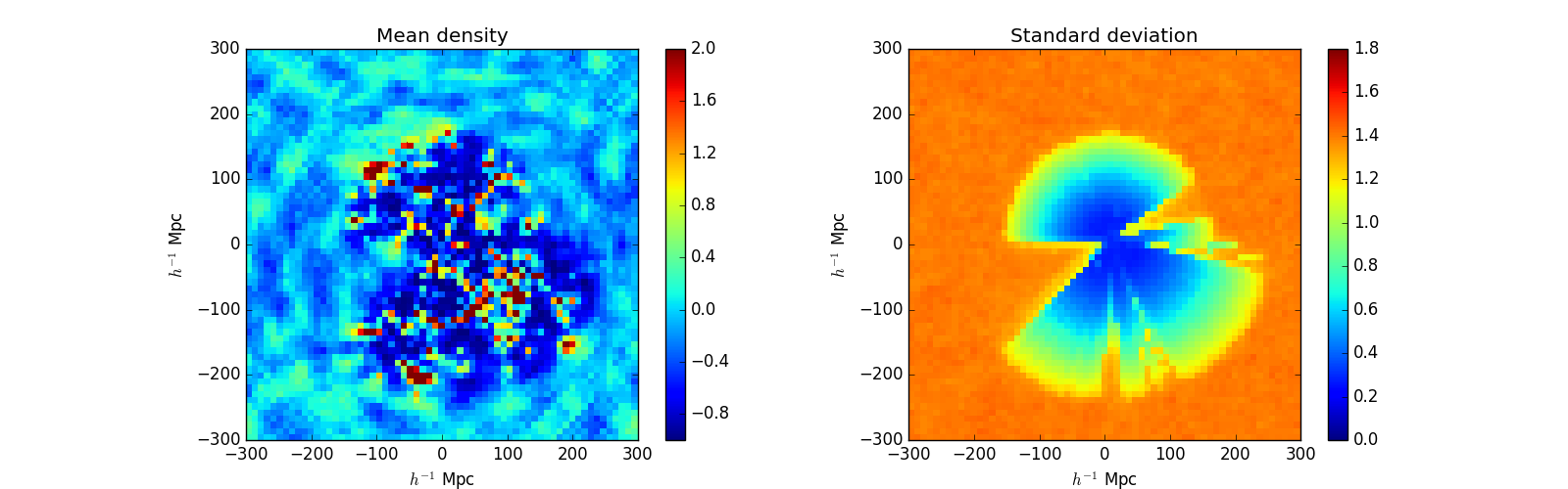
ax.set_title('Mean density')
ax.set_xlabel('$h^{-1}$ Mpc')
ax.set_ylabel('$h^{-1}$ Mpc')
fig.colorbar(im)

ax = fig.add_subplot(122)
im = ax.pcolormesh(ix[:,None].repeat(N,axis=1), ix[None,:].repeat(N,axis=0), density['scalars.s_field'][1],vmin=0,vmax=1.8)
ax.set_aspect('equal')
ax.set_xlim(-L/2,L/2)
ax.set_ylim(-L/2,L/2)
ax.set_xlabel('$h^{-1}$ Mpc')
ax.set_ylabel('$h^{-1}$ Mpc')
ax.set_title('Standard deviation')
fig.colorbar(im)

fig.savefig("density.png")

In this script we introduce read_chain_avg_dev (line 7) which allows to compute mean and standard deviation without loading the chain in memory. Additionally the slicer argument allows to only partially load the field. The step argument allows for thinning the chain by the indicator factor. In the above case we do not thin the chain. Also we request the field scalars.s_field (which contains the density field) and take only the plane x=32. The returned object is a named-columned object. Also, density[‘scalars.s_field’] is a [2,M0,…] array, with M0,… being the dimensions returned by the slicer function. The first slice is the mean field (as can be seen on line 18) and the second is the standard deviation (line 28).

Once the script is run we get the following pictures:

Density_tutorial1_ares.png

We can see that there are large scale features in the mean field (like ringing here). Though even in perfect conditions this feature could occur, this could also indicate a defect in the selection characterization process.

Running HADES

Hades3 is built at the same time as ares3. The final binary is located in $BUILD/src/hades3, which is the main HADES3 program. Again typing $BUILD/src/hades3 should give the following output:

setupMPI with threads
Initializing console.
[0/1] [DEBUG  ] INIT: MPI/FFTW
[STD    ]
[STD    ]                     /\_/\____,          ____________________________
[STD    ]           ,___/\_/\ \  ~     /                       HADES3
[STD    ]           \     ~  \ )   XXX
[STD    ]             XXX     /    /\_/\___,     (c) Jens Jasche 2012 - 2017
[STD    ]                \o-o/-o-o/   ~    /        Guilhem Lavaux 2014 - 2017
[STD    ]                 ) /     \    XXX        ____________________________
[STD    ]                _|    / \ \_/
[STD    ]             ,-/   _  \_/   \
[STD    ]            / (   /____,__|  )
[STD    ]           (  |_ (    )  \) _|
[STD    ]          _/ _)   \   \__/   (_
[STD    ]         (,-(,(,(,/      \,),),)
[STD    ] Please acknowledge XXXX
[0/1] [DEBUG  ] INIT: FFTW/WISDOM
[0/1] [INFO   ] Starting HADES3. rank=0, size=1
[0/1] [INFO   ] ARES3 base version c9e74ec93121f9d99a3b2fecb859206b4a8b74a3
[0/1] [ERROR  ] HADES3 requires exactly two parameters: INIT or RESUME as first parameter and the configuration file as second parameter.

Running BORG: a tutorial to perform a cosmological analysis

Downloading and Installing BORG

This note provides a step by step instruction for downloading and installing the BORG software package. This step-by-step instruction has been done using a MacBook Air running OS X El Capitan. I encourage readers to modify this description as may be required to install BORG on a different OS. Please indicate all necessary modifications and which OS was used.

Some Prerequisites

cmake≥ 3.10 automake libtool pkg-config gcc ≥ 7 , or intel compiler (≥ 2018), or Clang (≥ 7) wget (to download dependencies; the flag –use-predownload can be used to bypass this dependency if you already have downloaded the required files in the downloads directory)

Clone the repository from BitBucket

To clone the ARES repository execute the following git command in a console:

git clone --recursive git@bitbucket.org:bayesian_lss_team/ares.git

After the clone is successful, you shall change directory to ares, and execute:

bash get-aquila-modules.sh --clone

Ensure that correct branches are setup for the submodules using:

bash get-aquila-modules.sh --branch-set

If you want to check the status of the currently checked out ARES and its modules, please run:

bash get-aquila-modules.sh --status

You should see the following output:

!!!!!!!!!!!!!!!!!!!!!!!!!!!!!!!!!!!!!!!!!!!!!!!!!!!!!!!!!!!!!!!!!!!!!!!!
This script can be run only by Aquila members.
if your bitbucket login is not accredited the next operations will fail.
!!!!!!!!!!!!!!!!!!!!!!!!!!!!!!!!!!!!!!!!!!!!!!!!!!!!!!!!!!!!!!!!!!!!!!!!
Checking GIT status...

Root tree    (branch master) : good. All clear.
Module ares_fg  (branch master) : good. All clear.
Module borg (branch master) : good. All clear.
Module dm_sheet (branch master) : good. All clear.
Module hades    (branch master) : good. All clear.
Module hmclet   (branch master) : good. All clear.
Module python   (branch master) : good. All clear.

Building BORG

To save time and bandwidth it is advised to pre-download the dependencies that will be used as part of the building procedure. You can do that with

bash build.sh --download-deps

That will download a number of tar.gz which are put in the downloads/ folder.

Then you can configure the build itself:

bash build.sh --cmake CMAKE_BINARY --c-compiler YOUR_PREFERRED_C_COMPILER --cxx-compiler YOUR_PREFERRED_CXX_COMPILER --use-predownload

E.g. (This probably needs to be adjusted for your computer.):

bash build.sh --cmake /usr/local/Cellar/cmake/3.15.5/bin/cmake --c-compiler /usr/local/bin/gcc-9 --cxx-compiler /usr/local/bin/g++-9 --use-predownload

Once the configure is successful you should see a final output similar to this:

------------------------------------------------------------------

Configuration done.
Move to /Volumes/EXTERN/software/borg_fresh/ares/build and type 'make' now.
Please check the configuration of your MPI C compiler. You may need
to set an environment variable to use the proper compiler.

Some example (for SH/BASH shells):
- OpenMPI:
    OMPI_CC=/usr/local/bin/gcc-9
    OMPI_CXX=/usr/local/bin/g++-9
    export OMPI_CC OMPI_CXX

------------------------------------------------------------------

It tells you to move to the default build directory using cd build, after what you can type make. To speed up the compilation you can use more computing power by adding a -j option. For example

make -j4

will start 4 compilations at once (thus keep 4 cores busy all the time typically). Note, that the compilation can take some time.

Running a test example

The ARES repository comes with some standard examples for LSS analysis. Here we will use a simple standard unit example for BORG. From your ARES base directory change to the examples folder:

cd examples

To start a BORG run just execute the following code in the console:

../build/src/hades3 INIT borg_unit_example.ini

BORG will now execute a simple MCMC. You can interupt calculation at any time. To resume the run you can just type:

../build/src/hades3 RESUME borg_unit_example.ini

You need at least on the order of 1000 samples to pass the initial warm-up phase of the sampler. As the execution of the code will consume about 2GB of your storage, we suggest to execute BORG in a directory with sufficient free hard disk storage.

Analysing results

Now we will look at the out puts generated by the BORG run. Note, that you do not have to wait for the run to complete, but you can already investigate intermediate results while BORG still runs. BORG results are stored in two major HDF5 files, the restart and the mcmc files. The restart files contain all information on the state of the Markov Chain required to resume the Markov Chain if it has been interrupted. The restart file also contains static information, that will not change during the run, such as the data, selection functions and masks and other settings. The mcmc files contain the current state of the Markov Chain. They are indexed by the current step in the chain, and contain the current sampled values of density fields, power-spectra, galaxy bias and cosmological parameters etc.

Opening files

The required python preamble:

import numpy as np
import h5py as h5
import matplotlib.pyplot as plt
import ares_tools as at
%matplotlib inline

import warnings
warnings.filterwarnings("ignore")

Skipping VTK tools

Now please indicate the path where you stored your BORG run:

fdir='../testbed/'

Investigating the restart file

The restart file can be opened by

hf=h5.File(fdir+'restart.h5_0')

The content of the file can be investigated by listing the keys of the ‘scalar’ section

list(hf['scalars'].keys())

['ARES_version',
 'BORG_final_density',
 'BORG_version',
 'BORG_vobs',
 'K_MAX',
 'K_MIN',
 'L0',
 'L1',
 'L2',
 'MCMC_STEP',
 'N0',
 'N1',
 'N2',
 'N2_HC',
 'N2real',
 'NCAT',
 'NFOREGROUNDS',
 'NUM_MODES',
 'Ndata0',
 'Ndata1',
 'Ndata2',
 'adjust_mode_multiplier',
 'ares_heat',
 'bias_sampler_blocked',
 'borg_a_final',
 'borg_a_initial',
 'catalog_foreground_coefficient_0',
 'catalog_foreground_maps_0',
 'corner0',
 'corner1',
 'corner2',
 'cosmology',
 'forcesampling',
 'fourierLocalSize',
 'fourierLocalSize1',
 'galaxy_bias_0',
 'galaxy_bias_ref_0',
 'galaxy_data_0',
 'galaxy_nmean_0',
 'galaxy_sel_window_0',
 'galaxy_selection_info_0',
 'galaxy_selection_type_0',
 'galaxy_synthetic_sel_window_0',
 'gravity.do_rsd',
 'growth_factor',
 'hades_accept_count',
 'hades_attempt_count',
 'hades_mass',
 'hades_sampler_blocked',
 'hmc_Elh',
 'hmc_Eprior',
 'hmc_bad_sample',
 'hmc_force_save_final',
 'k_keys',
 'k_modes',
 'k_nmodes',
 'key_counts',
 'lightcone',
 'localN0',
 'localN1',
 'localNdata0',
 'localNdata1',
 'localNdata2',
 'localNdata3',
 'localNdata4',
 'localNdata5',
 'momentum_field',
 'nmean_sampler_blocked',
 'part_factor',
 'pm_nsteps',
 'pm_start_z',
 'powerspectrum',
 'projection_model',
 's_field',
 's_hat_field',
 'sigma8_sampler_blocked',
 'startN0',
 'startN1',
 'supersampling',
 'tCOLA',
 'total_foreground_blocked']

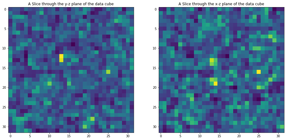
For example the input galaxy data can be viewed by:

data=np.array(hf['scalars/galaxy_data_0'])

#Plot data
fig, (ax1, ax2) = plt.subplots(1, 2,figsize=(16, 8))
ax1.set_title('A Slice through the y-z plane of the data cube')
im1=ax1.imshow(data[16,:,:])

ax2.set_title('A Slice through the x-z plane of the data cube')
im2=ax2.imshow(data[:,16,:])

plt.show()

Investigating MCMC files

MCMC files are indexed by the sample number $i_{samp}$. Each file can be opened separately. Suppose we want to open the $10$th mcmc file, then:

isamp=10 # sample number
fname_mcmc=fdir+"mcmc_"+str(isamp)+".h5"
hf=h5.File(fname_mcmc)

Inspect the content of the mcmc files

list(hf['scalars'].keys())

['BORG_final_density',
 'BORG_vobs',
 'catalog_foreground_coefficient_0',
 'cosmology',
 'galaxy_bias_0',
 'galaxy_nmean_0',
 'hades_accept_count',
 'hades_attempt_count',
 'hmc_Elh',
 'hmc_Eprior',
 'powerspectrum',
 's_field',
 's_hat_field']

Plotting density fields

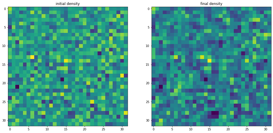
We can for instance be interested in plotting inferred initial and final density samples.

delta_in=np.array(hf['scalars/s_field'])
delta_fi=np.array(hf['scalars/BORG_final_density'])

fig, (ax1, ax2) = plt.subplots(1, 2,figsize=(16, 8))
ax1.set_title('initial density')
im1=ax1.imshow(delta_in[16,:,:])

ax2.set_title('final density')
im2=ax2.imshow(delta_fi[16,:,:])

plt.show()

Plotting the power-spectrum

The ARES repository provides some routines to analyse the BORG runs. A particularly useful routine calculates the posterior power-spectra of inferred initial density fields.

ss = at.analysis(fdir)

#Nbin is the number of modes used for the power-spectrum binning
opts=dict(Nbins=32,range=(0,ss.kmodes.max()))

#You can choose the sample numper
isamp=10
P=ss.compute_power_shat_spectrum(isamp, **opts)

kmode = 0.5*(P[2][1:]+P[2][:-1])
P_k   = P[0]

plt.loglog(kmode,P_k)
plt.xlabel('k [h/Mpc]')
plt.xlabel(r'$P(k)$')
plt.show()

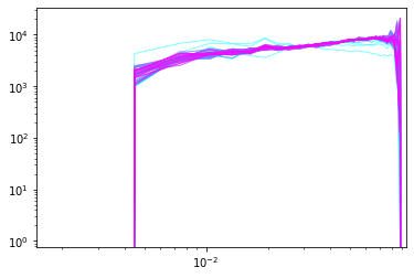
Monitoring power-spectrum warm-up phase

Rather than looking just at individual posterior sample power-spectra we can follow the evolution of power-spectra across the chain. Suppose you want to monitor the first 100 samples.

Nsamp=100
PPs=[]
for isamp in np.arange(Nsamp):
    PPs.append(ss.compute_power_shat_spectrum(isamp, **opts))


#plot power-spectra
color_idx = np.linspace(0, 1, Nsamp)
idx=0
for PP in PPs:
    plt.loglog(kmode,PP[0],alpha=0.5,color=plt.cm.cool(color_idx[idx]), lw=1)
    idx=idx+1
plt.xlim([min(kmode),max(kmode)])
plt.show()

Running BORG with simulation data

Pre-run test

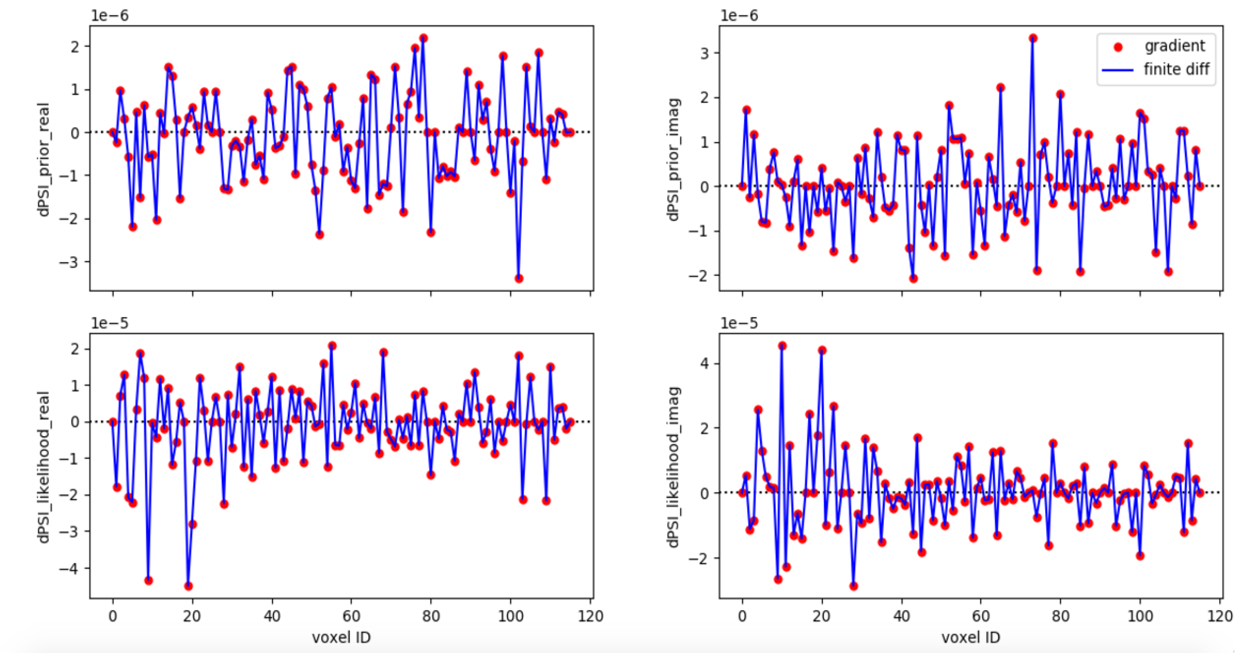
Gradient test

Run <ARES_REPO_DIR>/build.sh with ~~debug
Execute <BUILD_DIR>/libLSS/tests/test_gradient_<bias_model>
Grab dump.h5.
Plot analytical and numerical gradient (by finite difference), can use the script in <ARES_REPO_DIR>/scripts/check_gradients.py
Example:

Setup and tuning

ARES configuration file and input files

ARES configuration file:
- Documentation: here
- Set SIMULATION = True in ARES configuration file, <FILENAME>.ini.
- Set corner0, corner1, corner2 = 0.
- See, for example, ARES configuration file for BORG runs using SIMULATION data
Halo catalog:
- ASCII format: 5 columns (ID, $M_h$, $R_h$, spin, x, y, z, $v_x$, $v_y$, $v_z$). See, for example, Python scripts to convert AHF output to ASCII catalog for BORG.
- HDF5 format: similar to above. See, for example, Python scripts to convert AHF output to HDF5 catalog for BORG.
Trivial HEALPix mask where all pixels are set to 1 (choose approriate NSIDE for your BORG grid resolution).
Flat selection function in ASCII format. See, for example, Flat selection function file.

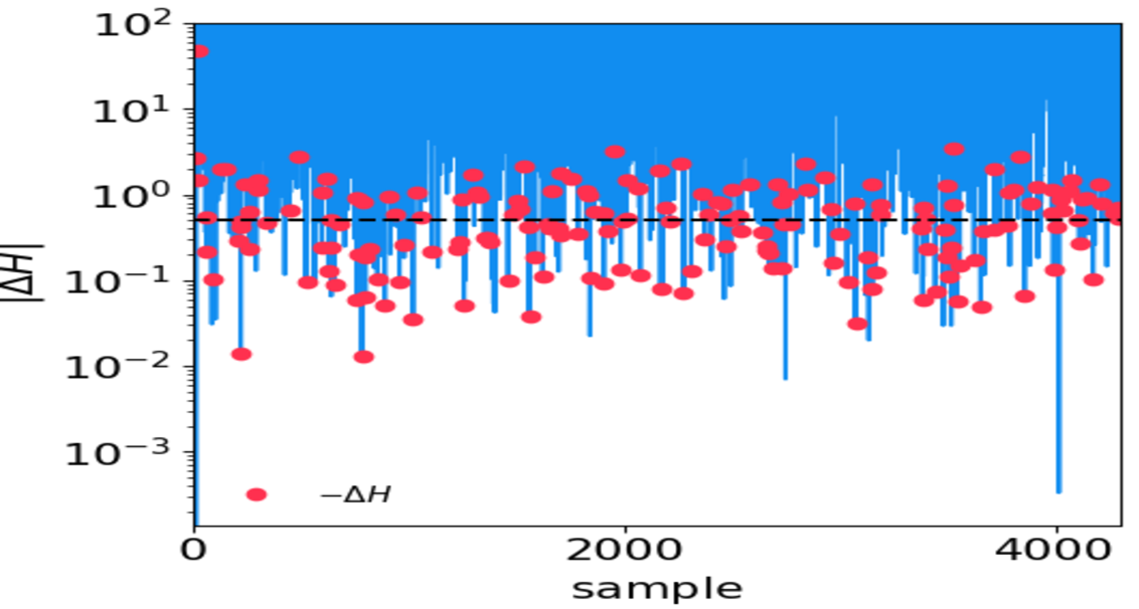
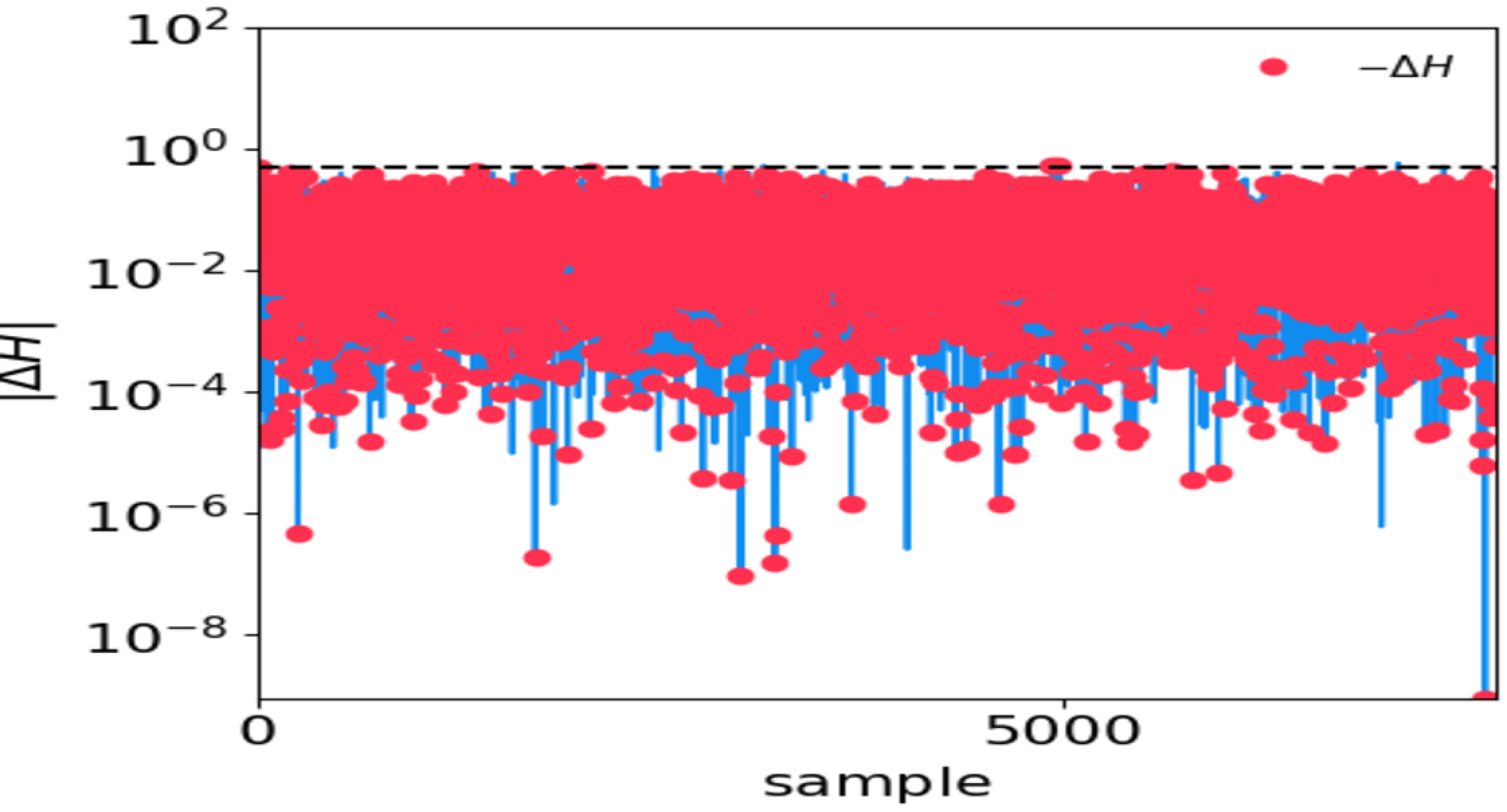
HMC performance tuning

Grab <OUTPUT_DIR>/hmc_performance.txt.
Plot $\Delta H$ and $|\Delta H|$.
Tune max_epsilon and max_timestep in the .ini file accordingly.
An example of bad HMC performance. The horizontal dashed line denotes $|\Delta H|=0.5$. Red dots denote negative $\Delta H$:

An example of good HMC performance:

After-run checks

Convergence check

Grab all <OUTPUT_DIR>/mcmc_<mcmc_identifier>.h5.
Plot $P_{mm, \mathrm{ini}}^s(k)$ vs. $P_{mm, \mathrm{ini}}^{\mathrm{theory}}(k)$.

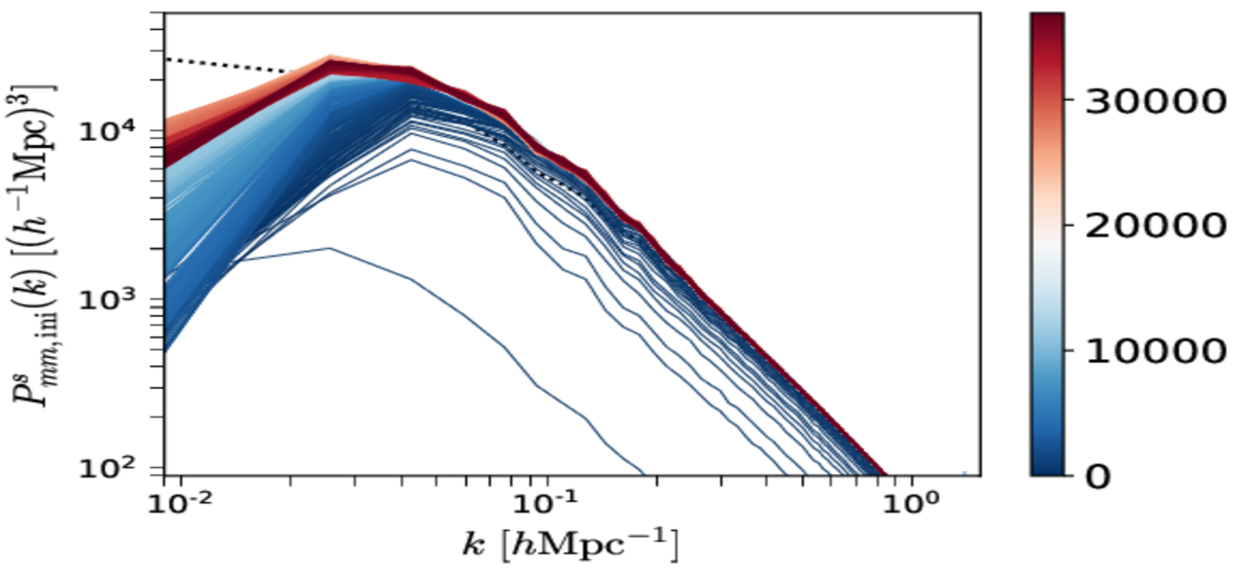
BORG_with_simulation_data_files/Pk_convergence.png

Correlation check

Compute noise residual in each BORG $s$-th sample as $\vec{\delta}_{\mathrm{res}}^s=\vec{\delta}_{m,\mathrm{ini}}^s-\left\langle\vec{\delta}_{m,\mathrm{ini}}\right\rangle_{s'}$.
Plot $r_{\mathrm{residual}}(\Delta s=s'-s)\equiv\frac{\mathrm{Cov}\left(\vec{\delta}_{\mathrm{res}}^s,\,\vec{\delta}_{\mathrm{res}}^{s'}\right)}{\sigma_s \sigma_{s'}}$.

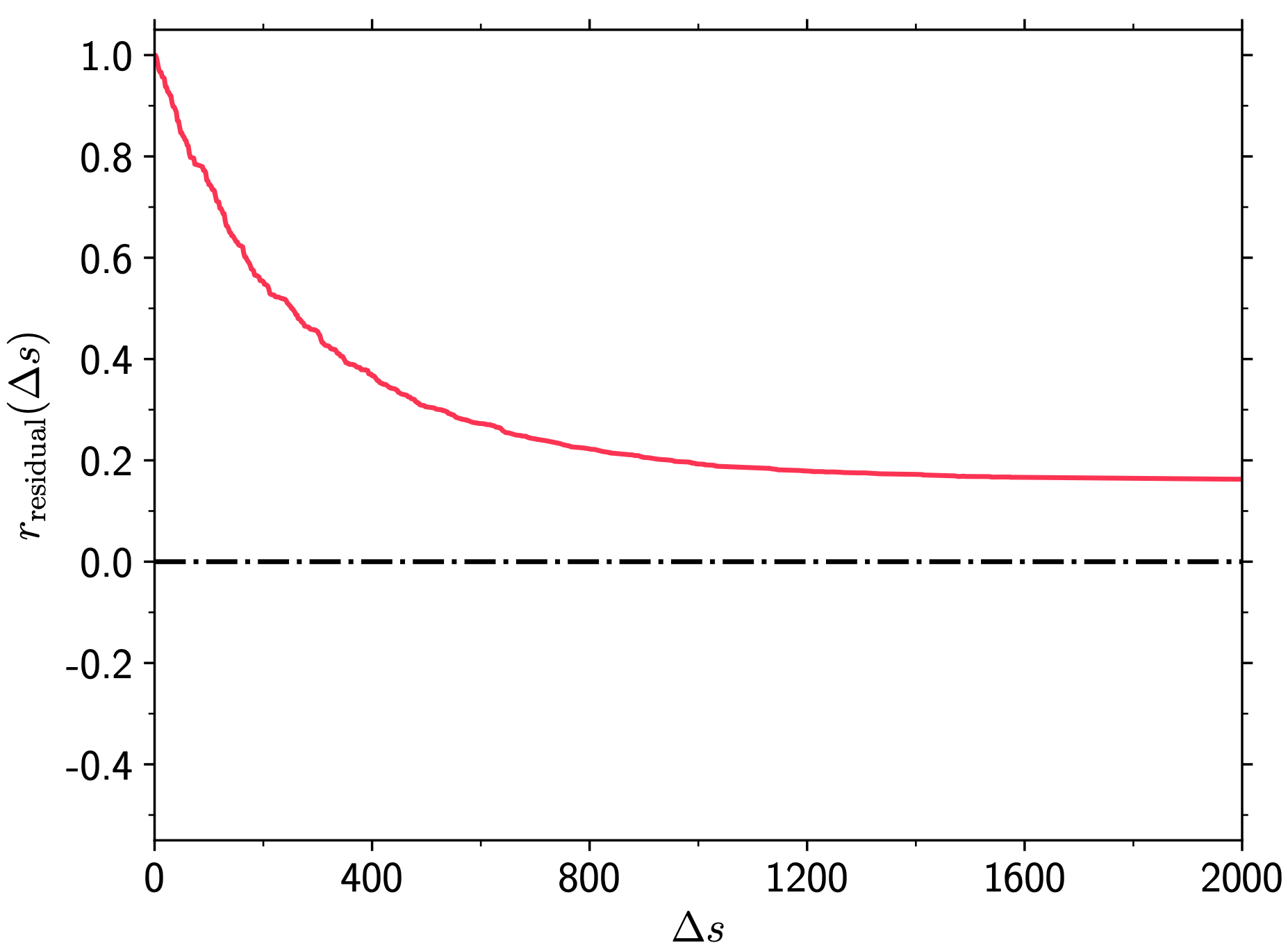
BORG_with_simulation_data_files/Residual_correlation_length.png