Postprocessing
Postprocessing scripts
ARES Plotting library
There is one repository that concentrate plotting routines and ready to use program to postprocess ARES MCMC chains. It is located at https://bitbucket.org/bayesian_lss_team/ares_visualization/. Please enrich it at the same time as this page.
show_log_likelihood.py
To be run in the directory containing the MCMC chain. Compute the power spectrum of initial conditions, binned correctly, for each sample and store it into a NPZ file. The output can be used by plot_power.py
plot_power.py
Contrast field in scatter plot
import numpy as np

dset_test=np.ones((32,32,32))

def contrast2cic(dset):
   Nbox=dset.shape[0]
   cic=np.zeros((Nbox,Nbox,Nbox))
   min_dset=min(dset.flatten())

   for m in range(Nbox):
      for k in range(Nbox):
          for j in range(Nbox):
            d=dset[m,k,j]
              cic[m][k][j]=int(np.floor((1+d)/(1+min_dset)))
   return cic

cic=contrast2cic(dset_test)
Acceptance rate
import matplotlib.pyplot as plt
import h5py

acceptance=[]
accept=0

for m in range(latest_mcmc()):
   f1=h5py.File('mcmc_'+str(m)+'.h5','r')
   accept=accept+np.array(f1['scalars/hades_accept_count'][0])
   acceptance.append(accept/(m+1))

plt.plot(acceptance)
plt.show()
Create gifs
import imageio
images = []
filenames=[]

for m in range(64,88):
   filenames.append('galaxy_catalogue_0x - slice '+str(m)+'.png')

for filename in filenames:
   images.append(imageio.imread(filename))

imageio.mimsave('datax.gif', images)
Scatter plot from galaxy counts in restart.h5
import h5py
import pyplot.matplotlib as plt

f=h5py.File('restart.h5_0','r')
data1=np.array(f['scalars/galaxy_data_0'])

xgrid=[]
ygrid=[]
zgrid=[]

for m in range(Nbox):
   for k in range(Nbox):
      for j in range(Nbox):
         if data1[m,k,j]!=0:
            xgrid.append(m)
            ygrid.append(k)
            zgrid.append(j)

fig = plt.figure()
ax = Axes3D(fig)
ax.view_init(0, 80)
ax.scatter(xgrid, ygrid, zgrid,s=1.5,alpha=0.2,c='black')
plt.show()
Plot data on mask
import numpy as np
import healpy

# Import your ra and dec from the data
# Then projscatter wants a specific transform
# wrt what BORG outputs

ra=np.ones(10)
dec=np.ones(10)

corr_dec=-(np.pi/2.0)*np.ones(len(ra))
decmask=corr_dec+dec
corr_ra=np.pi*np.ones(len(ra))
ramask=ra+corr_ra

map='WISExSCOSmask.fits.gz'
mask = hp.read_map(map)
hp.mollview(mask,title='WISE mock')
hp.projscatter(decmask,ramask,s=0.2)
Non-plotting scripts
Download files from remote server (with authentication):
from requests.auth import HTTPBasicAuth
import requests

def download_from_URL(o):
    URL='https://mysite.com/dir1/dir2/'+'filename_'+str(o)+'.h5'
    r = requests.get(URL, auth=HTTPBasicAuth('login', 'password'),allow_redirects=True)
    open('downloaded_file_'+str(o)+'.h5', 'wb').write(r.content)
    return None

for o in range(10000):
    download_from_URL(o)
This works for horizon with the login and password provided in the corresponding page.
Get latest mcmc_%d.h5 file from a BORG run
import os

def latest_mcmc():
   strings=[]
   for root, dirs, files in os.walk("."):
      for file in files:
         if file.startswith("mcmc_"):
            string=str(os.path.join(root, file))[7:]
            string=string.replace('.h5','')
            strings.append(int(string))
return max(strings)
But beware: we want the file before the latest one to not destroy the writing process in the restart files.
Template generator
Jens Jasche has started a specific repository that gather python algorithms to post-process the BORG density field to create predictive maps for other effects on the cosmic sky. The effects that has been implemented are the following:
CMB lensing
Integrated Sachs-Wolfe effect
Shapiro Time-delay
The repository is available on bitbucket here.
Tutorial: checking ARES outputs in python
We first import numpy (to handle arrays), h5py (to read hdf5 files) and matplotlib.pyplot (to plot density slices):
import numpy as np
import h5py as h5
import matplotlib.pyplot as plt
%matplotlib inline
We then load the hdf5 file with h5py:
fdir="./" # directory to the ARES outputs
isamp=0 # sample number
fname_mcmc="mcmc_"+str(isamp)+".h5"
hf=h5.File(fname_mcmc)
We can then list the datasets in the hdf5 file:
list(hf.keys())
['scalars']
list(hf['scalars'].keys())
['catalog_foreground_coefficient_0',
 'galaxy_bias_0',
 'galaxy_nmean_0',
 'powerspectrum',
 's_field',
 'spectrum_c_eval_counter']
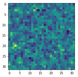
The density contrast is stored as ‘scalars/s_field’:
density=np.array(hf['scalars/s_field'])
We now plot a slice through the box:
plt.imshow(density[16,:,:])
The “restart” files contain a lot of useful information.
fname_restart=fdir+"restart.h5_0"
hf2=h5.File(fname_restart)
list(hf2.keys())
['galaxy_catalog_0', 'galaxy_kecorrection_0', 'random_generator', 'scalars']
list(hf2['scalars'].keys())
['ARES_version',
 'K_MAX',
 'K_MIN',
 'L0',
 'L1',
 'L2',
 'MCMC_STEP',
 'N0',
 'N1',
 'N2',
 'N2_HC',
 'N2real',
 'NCAT',
 'NFOREGROUNDS',
 'NUM_MODES',
 'adjust_mode_multiplier',
 'ares_heat',
 'bias_sampler_blocked',
 'catalog_foreground_coefficient_0',
 'catalog_foreground_maps_0',
 'corner0',
 'corner1',
 'corner2',
 'cosmology',
 'data_field',
 'fourierLocalSize',
 'fourierLocalSize1',
 'galaxy_bias_0',
 'galaxy_bias_ref_0',
 'galaxy_data_0',
 'galaxy_nmean_0',
 'galaxy_schechter_0',
 'galaxy_sel_window_0',
 'galaxy_selection_info_0',
 'galaxy_selection_type_0',
 'galaxy_synthetic_sel_window_0',
 'growth_factor',
 'k_keys',
 'k_modes',
 'k_nmodes',
 'key_counts',
 'localN0',
 'localN1',
 'messenger_field',
 'messenger_mask',
 'messenger_signal_blocked',
 'messenger_tau',
 'power_sampler_a_blocked',
 'power_sampler_b_blocked',
 'power_sampler_c_blocked',
 'powerspectrum',
 'projection_model',
 's_field',
 'sampler_b_accepted',
 'sampler_b_tried',
 'spectrum_c_eval_counter',
 'spectrum_c_init_sigma',
 'startN0',
 'startN1',
 'total_foreground_blocked',
 'x_field']
There we have in particular cosmological parameters:
cosmo=np.array(hf2['scalars/cosmology'])
print("h="+str(cosmo['h'][0])+", omega_m="+str(cosmo['omega_m'][0]))
h=0.6711, omega_m=0.3175
We also have the k modes to plot the power spectrum in our mcmc files:
k_modes=np.array(hf2['scalars/k_modes'])
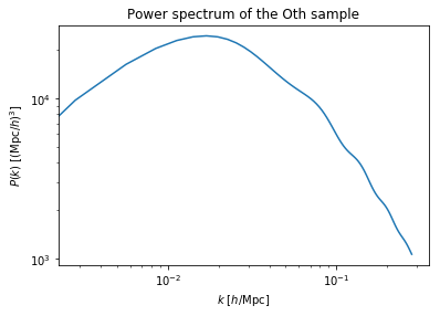
The power spectrum is stored in the mcmc files as ‘scalars/powerspectrum’:
powerspectrum=np.array(hf['scalars/powerspectrum'])
We can now make a plot.
plt.xlabel("$k$ [$h$/Mpc]")
plt.ylabel("$P(k)$ [$(\mathrm{Mpc}/h)^3$]")
plt.title("Power spectrum of the Oth sample")
plt.loglog(k_modes,powerspectrum)
Finally we close the hdf5 files.
hf.close()
hf2.close()
Tutorial: diagnostics of ARES/BORG chains
What this tutorial covers:
In this tutorial, we will cover how to do some basic plots of a BORG-run. These plots are useful for monitoring the burn-in progress of the run and diagnostics. Furthermore, how to plot BORG’s ability to sample/infer a specific parameter.
Prerequisites
Packages: numpy, h5py, pandas, matplotlib, tqdm What is assumed: I won’t go into much detail of how the python-code works. That said, this python-code is probably not the optimal way to do certain things, and I am sure it can be improved. BORG-Stuff: Have installed/compiled BORG as well as managed a first run. We will be using the data-products (the restart.h5_0-file and mcmc_#.h5-files)
Overview of tutorial - what are we producing
Galaxy projections
Statistics of the Ensemble density field
Burn-in of the powerspectra
Correlation matrix of the bias parameters
Trace plot and histogram of sampled parameter
Correlation length of a parameter
Acceptance Rate
Animations (gifs) of the density field and galaxy field
Take-aways/Summary - What can be used in the future?
The aim of this tutorial is to provide some tools to view the data-products that are in the mcmc-files, and to view features of the chain itself.
Don’t forget that this jupyter notebook can be exported to a .py-file!
We import some packages here. Note that we have ares_tools here, which is found under ares/scripts/ares_tools/. Move this to the working directory, or create a symbolic link (e.g. add to Python-path) in order to get this tutorial to work.
import os
import sys
import numpy as np
import h5py as h5
import pandas as pd
from tqdm import tqdm
import ares_tools as at

import matplotlib as mpl
import matplotlib.cm as cm
import matplotlib.pyplot as plt
from matplotlib import gridspec

mpl.rcParams['font.size'] = 15
Here we set our own colormap, can be fun if you want to customize your plots
import matplotlib.colors as mcolors

low = 'indigo'#
midlow = 'darkviolet'#
mid = 'darkgrey'
midhigh = 'gold'#
high = 'goldenrod' #
color_array = [low, midlow, mid, midhigh, high]
my_cmap = mcolors.LinearSegmentedColormap.from_list('my_cmap',color_array)
cm.register_cmap(cmap=my_cmap)
# LOAD FILES/CHECK FILES
startMC = 0

names=[]
PP=[]
Fmax=startMC
while True:
    try:
      os.stat("mcmc_%d.h5" % Fmax)
      names.append(Fmax)
      Fmax += mcDelta
    except:
      break
loc_names = list(names)
num = np.shape(names)[0]
print("Number of mcmc-files found: %d" % num)

restarts=[]
Gmax = 0
while True:
    try:
      os.stat("restart.h5_%d" % Gmax)
      restarts.append(Gmax)
      Fmax += mcDelta
    except:
      break
loc_restarts = list(restarts)
rnum = np.shape(restarts)[0]
print("Number of restart-files found: %d" % rnum)
Load some constants of the run from the restart-file:
#LOAD THE RESTART-FILE
filepath = "restart.h5_0"
restart_file = h5.File(filepath,'r')

#LOAD CONFIG OF RUN
N = restart_file['scalars/N0'][0]
NCAT = restart_file['scalars/NCAT'][0]
no_bias_params = (restart_file['scalars/galaxy_bias_0'][:]).shape[0]
restart_file.close()

#PREPARE GALAXY FIELD
gal_field = np.zeros((N,N,N))
restart_dens_field = np.zeros((N,N,N))

#STORE ALL OF THE GALAXIES
for r in np.arange(rnum):
    temp_restart = h5.File('restart.h5_%d' % r,'r')
    for i in np.arange(NCAT):
        gal_field[(r*N:(r+1)*N),:,:] += temp_restart['scalars/galaxy_data_%d' % i][:]
    restart_dens_field[(r*N:(r+1)*N),:,:] += temp_restart['scalars/BORG_final_density'][:]
    temp_restart.close()
print('Total number of galaxies: %d' % np.sum(gal_field))
Galaxy projection & ensemble density field: mean and standard deviation
In this plot, I have gathered the galaxy projection as well as ensemble statistics for the density field. The galaxy projection is a sum over all the galaxies in one direction at a time. We are viewing the input data (the galaxies) as a whole, which is found in the restart-file. With the ensemble statistics for the density field, we sum up all of the reconstructed density fields in the mcmc-files (mcmc_#.h5) and then compute the mean and the standard deviation of the field in each voxel.
The aim of these plots are to:
Check so that the galaxy data is fully within the datacube. If the datacube is misaligned with the galaxy data, we are not using all of the input data. This may sometimes be intended, but for most of the times we want to avoid this.
Check so that the reconstructed density fields coincide with the data-filled regions (i.e., where we have galaxies/data). We expect to have values distinct from the cosmic mean (usually zero) where we have data, and values close to the cosmic mean where we do not have data.
Check so that we have less variance inside the data-filled regions than outside the data-filled regions.
#PREPARE THE ENSEMBLE DENSITY FIELD HOLDER - FOR THE MEAN DENSITY FIELD
dens_fields = np.array(np.full((N,N,N),0),dtype=np.float64)

#COMPUTE THE MEAN-DENSITY FIELD
for idx in tqdm(np.arange(num)):
    mcmc_file = h5.File("mcmc_%d.h5" % idx,'r')
    temp_field = np.array(mcmc_file['scalars/BORG_final_density'][...],dtype=np.float64)
    dens_fields += temp_field
    mcmc_file.close()
mean_field = dens_fields/np.float64(num)


#PREPARE THE ENSEMBLE DENSITY FIELD HOLDER - FOR THE STANDARD DEVIATION DENSITY FIELD
dens_fields = np.array(np.full((N,N,N),0),dtype=np.float64)

#COMPUTE THE STANDARD DEVIATION DENSITY FIELD
for idx in tqdm(np.arange(num)):
    mcmc_file = h5.File("mcmc_%d.h5" % idx,'r')
    temp_field = np.array(mcmc_file['scalars/BORG_final_density'][...],dtype=np.float64)
    temp_field -= mean_field
    dens_fields += temp_field*temp_field
    mcmc_file.close()
std_field = np.sqrt(dens_fields/(num-1))
print(std_field)

#SAVE THE FIELDS
np.savez('projection_fields.npz',mean_field = mean_field,
         gal_field = gal_field,
         std_field = std_field,
         restart_dens_field = restart_dens_field)
Here we load the data from the previous step and produce projection plots
#LOAD DATA FROM THE .NPZ-FILES
data = np.load('projection_fields.npz')
mean_field = data['mean_field']
std_field = data['std_field']
gal_field = data['gal_field']
restart_dens_field = data['restart_dens_field']

#FIRST GALAXY PROJECTION IN THE X-DIRECTION
plt.figure(figsize=(20,20))
print('First subplot')
plt.subplot(3,3,1)
plt.title('No Galaxies: ' + str(np.sum(gal_field)))
proj_gal_1 = np.sum(gal_field,axis = 0)
im = plt.imshow(np.log(proj_gal_1),cmap=my_cmap)
clim=im.properties()['clim']
plt.colorbar()
plt.xlabel('Z')
plt.ylabel('Y')

#SECOND GALAXY PROJECTION IN THE Y-DIRECTION
print('Second subplot')
plt.subplot(3,3,4)
proj_gal_2 = np.sum(gal_field,axis = 1)
plt.imshow(np.log(proj_gal_2), clim=clim,cmap=my_cmap)
plt.colorbar()
plt.xlabel('Z')
plt.ylabel('X')

#THIRD GALAXY PROJECTION IN THE Z-DIRECTION
print('Third subplot')
plt.subplot(3,3,7)
proj_gal_3 = np.sum(gal_field,axis = 2)
plt.imshow(np.log(proj_gal_3), clim=clim,cmap=my_cmap)
plt.colorbar()
plt.xlabel('Y')
plt.ylabel('X')

#FIRST ENSEMBLE DENSITY MEAN IN THE X-DIRECTION
print('Fourth subplot')
plt.subplot(3,3,2)
plt.title("Ensemble Mean Density field")
proj_dens_1 = np.sum(mean_field,axis = 0)
im2 = plt.imshow(np.log(1+proj_dens_1),cmap=my_cmap)
clim=im2.properties()['clim']
plt.colorbar()
plt.xlabel('Z')
plt.ylabel('Y')

#SECOND ENSEMBLE DENSITY MEAN IN THE Y-DIRECTION
print('Fifth subplot')
plt.subplot(3,3,5)
proj_dens_2 = np.sum(mean_field,axis = 1)
plt.imshow(np.log(1+proj_dens_2), clim=clim,cmap=my_cmap)
plt.colorbar()
plt.xlabel('Z')
plt.ylabel('X')

#THIRD ENSEMBLE DENSITY MEAN IN THE Z-DIRECTION
print('Sixth subplot')
plt.subplot(3,3,8)
proj_dens_3 = np.sum(mean_field,axis = 2)
plt.imshow(np.log(1+proj_dens_3), clim=clim,cmap=my_cmap)
plt.colorbar()
plt.xlabel('Y')
plt.ylabel('X')

#FIRST ENSEMBLE DENSITY STD. DEV. IN THE X-DIRECTION
print('Seventh subplot')
plt.subplot(3,3,3)
plt.title('Ensemble Std. Dev. Dens. f.')
proj_var_1 = np.sum(std_field,axis = 0)
im3 = plt.imshow(np.log(1+proj_var_1),cmap=my_cmap)
clim=im3.properties()['clim']
plt.colorbar()
plt.xlabel('Z')
plt.ylabel('Y')

#SECOND ENSEMBLE DENSITY STD. DEV. IN THE Y-DIRECTION
print('Eighth subplot')
plt.subplot(3,3,6)
proj_var_2 = np.sum(std_field,axis = 1)
plt.imshow(np.log(1+proj_var_2), clim=clim,cmap=my_cmap)
plt.colorbar()
plt.xlabel('Z')
plt.ylabel('X')

#THIRD ENSEMBLE DENSITY STD. DEV. IN THE Z-DIRECTION
print('Ninth subplot')
plt.subplot(3,3,9)
proj_var_3 = np.sum(std_field,axis = 2)
plt.imshow(np.log(1+proj_var_3), clim=clim,cmap=my_cmap)
plt.colorbar()
plt.xlabel('Y')
plt.ylabel('X')

plt.savefig('GalaxyProjection.png')
plt.show()
Burn-in power spectra
This plot computes and plots the powerspectrum for each of the mcmc-file together with the reference (or “true”) powerspectrum. In the bottom plot, we divide each powerspectrum with the reference powerspectrum, in order to see how much they deviate.
We expect that the powerspectra of the mcmc-files “rise” throughout the run to the reference powerspectrum. The colormap is added to more easily see the different powerspectra of the run.
# COMPUTE BURN-IN P(k) AND SAVE TO FILE
ss = at.analysis(".")
opts=dict(Nbins=N,range=(0,ss.kmodes.max()))
Pref = ss.rebin_power_spectrum(startMC, ==opts)

PP = []
loc_names = list(names)

mcDelta = 1
step_size = 1
print('Computing Burn-In Powerspectra')
for i in tqdm(loc_names[0::step_size]):
    PP.append(ss.compute_power_shat_spectrum(i, ==opts))

bins = 0.5*(Pref[2][1:]+Pref[2][:-1])

suffix = 'test'
np.savez("power_%s.npz" % suffix, bins=bins, P=PP, Pref=Pref)
print('File saved!')
Plotting routines
from mpl_toolkits.axes_grid1.inset_locator import inset_axes
# LOAD DATA
suffix = 'test'
x=np.load("power_%s.npz" % suffix, allow_pickle=True)
sampled_pk = np.array([x['P'][i,0][:] for i in range(len(x['P']))]).transpose()

# PREPARE FIRST SUBPLOT
plt.figure(figsize=(10,10))
gs = gridspec.GridSpec(2, 1, height_ratios=[2, 1])

p = plt.subplot(gs[0])


# PLOT THE BURN-IN POWERSPECTRA
no_burn_ins = (sampled_pk).shape[1]
color_spectrum = iter(my_cmap(np.linspace(0,1,no_burn_ins))); #Here we include the colormap
for j in np.arange(no_burn_ins):
    p.loglog(x['bins'], sampled_pk[:,j], color = next(color_spectrum), alpha=0.25)

# PLOT THE REFERENCE POWERSPECTRUM
p.loglog(x['bins'], x['Pref'][0],color='k',lw=0.5,
        label = "Reference powerspectrum")

# SOME CONTROL OVER THE AXES
#cond = x['Pref'][0] > 0
#xb = x['bins'][cond]
#p.set_xlim(0.01, 0.2)
#p.set_ylim(1,0.9*1e5)

# LABELLING
plt.xlabel(r'$k \ [\mathrm{Mpc} \ h^{-1} ]$')
plt.ylabel(r'$P(k) \ [\mathrm{Mpc^{3}} \ h^{-3} ]$')
plt.title('Powerspectrum Burn-in for run: ' + suffix)
p.tick_params(bottom = False,labelbottom=False)

plt.legend()

# SET THE COLORBAR MANUALLY
norm = mpl.colors.Normalize(vmin=0,vmax=2)
sm = plt.cm.ScalarMappable(cmap=my_cmap, norm=norm)
sm.set_array([])
cbaxes = inset_axes(p, width="30%", height="3%", loc=6)
cbar = plt.colorbar(sm,cax = cbaxes,orientation="horizontal",
                    boundaries=np.arange(-0.05,2.1,.1))
cbar.set_ticks([0,1,2])
cbar.set_ticklabels([0,int(no_burn_ins/2),no_burn_ins])


# PREPARE THE SECOND PLOT, THE ERROR PLOT
p2 = plt.subplot(gs[1], sharex = p)

color_spectrum = iter(my_cmap(np.linspace(0,1,no_burn_ins)));
# PLOT THE ALL THE SAMPLED/RECONSTRUCTED POWERSPECTRA DIVIDED BY THE REFERENCE POWERSPECTRUM
for j in np.arange(no_burn_ins):
    p2.plot(x['bins'],sampled_pk[:,j]/(x['Pref'][0]),color = next(color_spectrum),alpha = 0.25)
# PLOT THE REFERENCE PLOT
p2.plot(x['bins'],(x['Pref'][0])/(x['Pref'][0]), color = 'k',lw = 0.5)

# SOME CONTROL OF THE AXES AND LABELLING
p2.set_yscale('linear')
#p2.set_ylim(0,2)
#plt.yticks(np.arange(0.6, 1.6, 0.2))
plt.xlabel(r'$k \ [\mathrm{Mpc} \ h^{-1} ]$')
plt.ylabel(r'$P(k)/P_{\mathrm{ref}}(k) $')
#plt.subplots_adjust(hspace=.0)
plt.savefig("burnin_pk.png")
plt.show()
Correlation matrix
Bias parameters are parameters of the galaxy bias model. While these are treated as nuisance parameters (i.e. they are required for the modelling procedure but are integrated out as they are not of interest) it’s important to check if there are internal correlations in the model. If there are internal correlations, we run the risk of “overfitting” the model, e.g. by having a bunch of parameters which do not add new information, but give rise to redundancies. An uncorrelated matrix suggests independent parameters, which is a good thing.
While I have only used bias parameters in this example, it is a good idea to add cosmological parameters (which are sampled!) to this matrix. Thereby, we can detect any unwanted correlations between inferred parameters and nuisance parameters.
# CORR-MAT
#A MORE FLEXIBLE WAY TO DO THIS? NOT HARDCODE THE BIAS MODEL OF CHOICE....?

bias_matrix = np.array(np.full((num,NCAT,no_bias_params+1),0),dtype=np.float64)
#num - files
#NCAT - catalogs
#no_bias_params = number of bias parameters
df = pd.DataFrame()
"""
# If you have an array of a sampled parameter (how to get this array, see next section),
# then you can add it to the correlation matrix like below:
df['Name_of_cosmo_param'] = sampled_parameter_array
"""
for i in tqdm(np.arange(num)):
    mcmc_file = h5.File("mcmc_%d.h5" % i,'r')
    for j in np.arange(NCAT):
        for k in np.arange(no_bias_params+1):
            if k == 0:
                bias_value = mcmc_file['scalars/galaxy_nmean_%d' % j][0]
            else:
                bias_value = mcmc_file['scalars/galaxy_bias_%d' % j][k-1]
            bias_matrix[i,j,k] = bias_value
    mcmc_file.close()

for j in np.arange(NCAT):
        for k in np.arange(no_bias_params+1):
            if k == 0:
                column_name = r"$\bar{N}^{%s}$" % j
            else:
                 column_name = (r"$b_{0}^{1}$".format(k,j))
            df[column_name]=bias_matrix[:,j,k]
#print(df) #PRINT THE RAW MATRIX

# Save the DataFrame
df.to_csv('bias_matrix.txt', sep=' ', mode='a')

f = plt.figure(figsize=(15,15))
plt.matshow(df.corr(), fignum=f.number, cmap=my_cmap, vmin=-1, vmax=1)
plt.xticks(range(df.shape[1]), df.columns, fontsize=14, rotation=45)
plt.yticks(range(df.shape[1]), df.columns, fontsize=14)
cb = plt.colorbar()
cb.ax.tick_params(labelsize=15)
#plt.title(title, fontsize=30);
plt.show()
plt.savefig('corrmat.png')
Trace-histogram
BORG can infer cosmological parameters and sample these throughout the run. One way to visualize BORG’s constraining power is to use trace plots and/or histograms. Basically, we gather the sampled values from each mcmc-file, store them to an array, and plot each value vs. step number (trace-plot) as well as the histogram of the distribution.
If the “true” value is known (for instance in mock runs), it can be added and plotted in the example below.
Also note, the example below is done on an array of bias parameters: change this to an array of a cosmological parameter.
from matplotlib.patches import Rectangle

def trace_hist(array_of_sampling_parameter,true_param=None, name_of_file='test'):

# =============================================================================
#      Compute statistics
# =============================================================================
    mean = np.mean(array_of_sampling_parameter)
    sigma = np.sqrt(np.var(array_of_sampling_parameter))

    xvalues = np.linspace(0,num-1,num)
    mean_sampled = mean*np.ones(num)

# =============================================================================
#     Trace-plot
# =============================================================================
    plt.figure(figsize=(15,10))
    ax1 = plt.subplot(2, 1, 1)
    plt.plot(xvalues,array_of_sampling_parameter,
             label = "Sampled Parameter Values",color = low,)

    if true_param != None:
        sampled_true_line = true_param*np.ones(num)
        plt.plot(xvalues,sampled_true_line,'--',color = midhigh,
                 label = "True value of Sampled Parameter")
    plt.plot(xvalues,mean_sampled, '-.',color = mid,
             label = "True value of Sampled Parameter")

    plt.xlabel(r'$\mathrm{Counts}$',size=30)
    plt.ylabel("Sampled Parameter",size=30,rotation=90)
    plt.legend()

# =============================================================================
#     Histogram
# =============================================================================

    plt.subplot(2,1, 2)
    (n, bins, patches) = plt.hist(array_of_sampling_parameter,bins = 'auto',color = low)
    samp_line = plt.axvline(mean, color=midhigh, linestyle='-', linewidth=2)

    if true_param != None:
        true_line = plt.axvline(true_param, color=mid, linestyle='--', linewidth=2)

    sigma_line = plt.axvline(mean+sigma,color = midlow, linestyle='-', linewidth=2)
    plt.axvline(mean-sigma,color = midlow, linestyle='-', linewidth=2)

    extra = Rectangle((0, 0), 1, 1, fc="w", fill=False, edgecolor='none', linewidth=0)
    if true_param != None:
        plt.legend([samp_line,true_line,sigma_line,extra, extra, extra],
                   ('Sampled$','True$',
                   '$1\sigma$ Interval',
                   '$N_{total}$: ' + str(num),
                    "$\mu$: "+str(round(mean,3)),
                    "$\sigma$: "+str(round(sigma,3))))
    else:
        plt.legend([samp_line,sigma_line,extra, extra, extra],
                   ('Sampled$',
                   '$1\sigma$ Interval',
                   '$N_{total}$: ' + str(num),
                    "$\mu$: "+str(round(mean,3)),
                    "$\sigma$: "+str(round(sigma,3))))

    """
    #HERE WE INCLUDE A SUMMARY STATISTICS STRING IN THE PLOT, OF THE SAMPLED PARAMETER
    x_pos = int(-1.5*int(sigma))
    summary_string = 'Sampled value = ' + str(round(mean,2)) +'$\pm$'+str(round(sigma,2))
    plt.text(x_pos, int(np.sort(n)[-3]), summary_string, fontsize=30)
    """


    plt.savefig('trace_hist_%s.png' % name_of_file)
    plt.show()

    plt.clf()


"""
# Here is an example of how to collect a
# sampled parameter from the mcmc-files

sampled_parameter_array = np.zeros(num)
cosmo_index = 1 #The index of the parameter of interest

for idx in tqdm(np.arange(num)):
    mcmc_file = h5.File("mcmc_%d.h5" % idx,'r')
    sampled_parameter_array[idx] = mcmc_file['scalars/cosmology'][0][cosmo_index]
    mcmc_file.close()
trace_hist(sampled_parameter_array)
"""


trace_hist(bias_matrix[:,1,1])
Correlation length
This plot demonstrates the correlation length of the chain, i.e. how many steps it takes for the sampling chain to become uncorrelated with the initial value. It gives some insight into “how long” the burn-in procedure is.
def correlation_length(array_of_sampling_parameter):
    # COMPUTES THE CORRELATION LENGTH
    autocorr = np.fft.irfft( (
        np.abs(np.fft.rfft(
            array_of_sampling_parameter - np.mean(array_of_sampling_parameter))) )**2 )
    zero_line = np.zeros((autocorr/autocorr[0]).shape)

    # PLOT THE CORRELATION LENGTH
    fig = plt.figure(figsize = (15,10))
    plt.plot(autocorr/autocorr[0],color = low)
    plt.plot(zero_line, 'r--',color = mid)
    Fmax=num
    mcDelta=1
    plt.xlim(0,Fmax/(2*mcDelta))
    plt.ylabel(r'$\mathrm{Correlation}$')
    plt.xlabel(r'$\mathrm{n \ (Step \ of \ mcmc \ chain)}$')
    plt.savefig('corr.png')
    plt.show()

# Runs the function on one of the bias-parameters
# -> adjust this call as in the trace-histogram field!
correlation_length(bias_matrix[:,1,1])
Acceptance rate
A way to visualize “how well” BORG manages to generate samples. A high rate of trials suggests that BORG is struggling and requires many runs to generate a sample. We expect that the acceptance rate is high at the start of the run then decreases over the course of the burn-in until it fluctuates around a certain value.
THIS PLOT IS NOT CORRECT YET!
# ACCEPTANCE-RATE
acc_array = np.full((num),0)
# GET THE ACCEPTANCE COUNTS FROM THE FILES
for i in np.arange(num):
    mcmc_file = h5.File("mcmc_%d.h5" % idx,'r')
    acceptance_number = mcmc_file['scalars/hades_accept_count'][0]
    acc_array[i] = acceptance_number

# COMPUTE THE MEAN SO THAT IT CAN BE INCLUDED INTO THE PLOT
mean_rate = np.mean(acc_array)
xvalues = np.linspace(0,num-1,num)
mean_acc = mean_rate*np.ones(num)

# PLOT THE FINDINGS
fig = plt.figure(figsize = (15,10))
plt.scatter(xvalues,acc_array,color = low, label = "Acceptance Rate")
plt.plot(xvalues,mean_acc, '-.',color = mid,
     label = "Mean Acceptance Rate")
plt.ylabel(r'$\mathrm{Acceptance}$')
plt.xlabel(r'$\mathrm{n \ (Step \ of \ mcmc \ chain)}$')
plt.savefig('acceptance_rate.png')
plt.show()
Animations/Gif-generator
A fun way to view the data is the use gifs. In this example, I’m slicing up the density field and the galaxy field (in three different directions of the data cube), saving each image (with imshow), then adding them to a gif.
First, we save the slices of the fields to a folder:
def density_slices(dens_field,catalog):
    # CREATE THE DIRECTORY TO SAVE SLICES
    os.system('mkdir %s' % catalog)

    # STORE THE MAX- AND MIN-POINTS FOR THE COLORBARS -> THIS CAN BE ADJUSTED
    dens_max = np.log(1+np.max(dens_field))
    dens_min = np.log(1+np.min(dens_field))

    # SAVE THE DENSITY SLICES
    for i in np.arange(N):
        plt.figure(figsize=(20,20))

        plt.imshow(np.log(1+dens_field[i,:,:]),
                   cmap = my_cmap,vmin = dens_min, vmax = dens_max)
        plt.title('X-Y Cut')
        plt.colorbar()
        plt.savefig(catalog+"/slice_X_Y_" + str(i) + ".png")
        plt.clf()


        plt.imshow(np.log(1+dens_field[:,i,:]),
                   cmap = my_cmap,vmin = dens_min, vmax = dens_max)
        plt.title('X-Z Cut')
        plt.colorbar()
        plt.savefig(catalog+"/slice_X_Z_" + str(i) + ".png")
        plt.clf()

        plt.imshow(np.log(1+dens_field[:,:,i]),
                   cmap = my_cmap,vmin = dens_min, vmax = dens_max)
        plt.title('Y-Z Cut')
        plt.colorbar()
        plt.savefig(catalog+"/slice_Y_Z_" + str(i) + ".png")
        plt.clf()


        plt.close()
    return

# RUN THE FUNCTION FOR THREE DIFFERENT FIELDS
density_slices(restart_dens_field,'dens_slices')
density_slices(gal_field,"gal_slices")
density_slices(mean_field,"mean_slices")
We generate the gifs below
import imageio
images1 = []
images2 = []
images3 = []
images4 = []
images5 = []
images6 = []
images7 = []
images8 = []
images9 = []

for i in np.arange(N):
    images1.append(imageio.imread("gal_slices/slice_X_Z_%d.png" % i))
    images2.append(imageio.imread("gal_slices/slice_X_Y_%d.png" % i))
    images3.append(imageio.imread("gal_slices/slice_Y_Z_%d.png" % i))
    images4.append(imageio.imread("dens_slices/slice_X_Z_%d.png" % i))
    images5.append(imageio.imread("dens_slices/slice_X_Y_%d.png" % i))
    images6.append(imageio.imread("dens_slices/slice_Y_Z_%d.png" % i))
    images7.append(imageio.imread("mean_slices/slice_X_Z_%d.png" % i))
    images8.append(imageio.imread("mean_slices/slice_X_Y_%d.png" % i))
    images9.append(imageio.imread("mean_slices/slice_Y_Z_%d.png" % i))

imageio.mimsave('gal_X_Z.gif', images1)
imageio.mimsave('gal_X_Y.gif', images2)
imageio.mimsave('gal_Y_Z.gif', images3)

imageio.mimsave('dens_X_Z.gif', images4)
imageio.mimsave('dens_X_Y.gif', images5)
imageio.mimsave('dens_Y_Z.gif', images6)

imageio.mimsave('mean_X_Z.gif', images7)
imageio.mimsave('mean_X_Y.gif', images8)
imageio.mimsave('mean_Y_Z.gif', images9)
Tutorial: generating constrained simulations from HADES
Get the source
First you have to clone the bitbucket repository
git@bitbucket.org:bayesian_lss_team/borg_constrained_sims.git
Ensure that you have the package H5PY and numexpr installed.
How to run
If you run “python3 gen_ic.py -h” it will print the following help:
usage: gen_ic.py [-h] --music MUSIC [--simulator SIMULATOR] [--sample SAMPLE]
                 [--mcmc MCMC] [--output OUTPUT] [--augment AUGMENT]

optional arguments:
  -h, --help            show this help message and exit
  --music MUSIC         Path to music executable
  --simulator SIMULATOR
                        Which simulator to target (Gadget,RAMSES,WHITE)
  --sample SAMPLE       Which sample to consider
  --mcmc MCMC           Path of the MCMC chain
  --output OUTPUT       Output directory
  --augment AUGMENT     Factor by which to augment small scales
All arguments are optional except “music” if it is not available in your PATH.
The meaning of each argument is the following:
music: Full path to MUSIC executable
simulator: Type of simulator that you wish to use. It can either be
WHITE, if you only want the ‘white’ noise (i.e. the Gaussian random number, with variance 1, which are used to generate ICs)
Gadget, for a gadget simulation with initial conditions as Type 1
RAMSES, for a ramses simulation (Grafic file format)
sample: Give the integer id of the sample in the MCMC to be used to generate ICs.
output: the output directory for the ICs
augment: whether to increase resolution by augmenting randomly the small scales (with unconstrained gaussian random numbers of variance 1). This parameter must be understood as a power of two multiplier to the base resolution. For example, ‘augment 2’ on a run at 256 will yield a simulation at 512. ‘augment 4’ will yield a simulation at 1024.
Generating initial conditions
TO BE IMPROVED
The main script can be found
here,
which generates ICs for one or a small number of steps in the MCMC
chain. You will need all the restart_* files, along with the mcmc_*
files of the step you want to analyse. You also need the Music
executable. Using src.bcs, the default is to generate ICs over the
entire simulation volume, with resolution increased by a factor of
fac_res (i.e. white noise generated up to this scale). If you set
select_inner_region=True then ICs are generated over only the
central half of the simulation volume, which effectively doubles your
resolution. An alternative is to use src.bcs_zoom, which instead zooms
in on the central sphere with radius and resolution as specified in that
script. In this case fac_res is irrelevant. Besides the properties
of the ellipse, the relevant parameter is the number in levelmax which
is the resolution with which you want to zoom in (e.g. if you start with
a \(256^3\) grid [levelmin=8], specifying levelmax=11 will
mean the zoom region starts at \(2048^3\) resolution). For either
script you can choose to generate ICs for either the Ramses or Gadget
simulators.
Result
Gadget
You will find a “gadget_param.txt” in the output directory and a file called ic.gad in the subdirectory “ic”. The log of the generation is in “white_noise/”
Ramses
Clumpfinding on the fly
There is a merger tree patch in Ramses which does halo-finding and
calculates merger trees as the simulation runs. The code is in
patch/mergertree in the ramses folder where there is also some
documentation. The halos are calculated and linked at each of the
specified outputs of the simulation, so for the merger trees to be
reliable these outputs must be fairly frequent. The most conservative
choice is to have an output every coarse time step. The mergertree patch
is activated by specifying clumpfind=.true. in the run_params block, and
adding a clumpfind_params block to specify the parameters of the
clumpfinding. The extra files that this generates at each output are
halo_* (properties of the halos), clump_* (properties of the clumps,
essentially subhalos; this should include all the halos as well),
mergertree_* (information on the connected halos across the timesteps)
and progenitor_data_* (which links the halos from one step to the
next). If you wish to store the merger tree information more frequently
than the full particles (restart) information, you can hack the code in
amr/output_amr to only output the part_*, amr_* and
grav_* files on some of the outputs (specified for example by the
scale factor aexp). You can also hack the code in
patch/mergertree/merger_tree.py to remove for example the
clump_* files (if you only want to keep main halos), and/or remove
the progenitor_data_* files before the preceding snapshot when they
are no longer necessary. Finally, you may wish to concatenate the
remaining files (e.g. mergertree_* and halo_*) over all the
processors.
Example namelist
&RUN_PARAMS
cosmo=.true.
pic=.true.
poisson=.true.
hydro=.false.
nrestart=0
nremap=20
nsubcycle=1,1,1,1,20*2
ncontrol=1
clumpfind=.true.
verbose=.false.
debug=.false.
/

&INIT_PARAMS
aexp_ini=0.0142857
filetype='grafic'
initfile(1)='/cosma7/data/dp016/dc-desm1/Ramses_8600/ic/ramses_ic/level_008'
initfile(2)='/cosma7/data/dp016/dc-desm1/Ramses_8600/ic/ramses_ic/level_009'
initfile(3)='/cosma7/data/dp016/dc-desm1/Ramses_8600/ic/ramses_ic/level_010'
initfile(4)='/cosma7/data/dp016/dc-desm1/Ramses_8600/ic/ramses_ic/level_011'
/

&AMR_PARAMS
ngridmax=3500000
npartmax=8000000
levelmin=8
levelmax=19
nexpand=0,0,20*1
/

&REFINE_PARAMS
m_refine=30*8.
mass_cut_refine=2.32831e-10
ivar_refine=0
interpol_var=0
interpol_type=2
/

&CLUMPFIND_PARAMS
!max_past_snapshots=3
relevance_threshold=3   ! define what is noise, what real clump
density_threshold=80    ! rho_c: min density for cell to be in clump
saddle_threshold=200    ! rho_c: max density to be distinct structure
mass_threshold=100      ! keep only clumps with at least this many particles
ivar_clump=0            ! find clumps of mass density
clinfo=.true.           ! print more data
unbind=.true.           ! do particle unbinding
nmassbins=100           ! 100 mass bins for clump potentials
logbins=.true.          ! use log bins to compute clump grav. potential
saddle_pot=.true.       ! use strict unbinding definition
iter_properties=.true.  ! iterate unbinding
conv_limit=0.01         ! limit when iterated clump properties converge
make_mergertree=.true.
nmost_bound=200
make_mock_galaxies=.false.
/

&OUTPUT_PARAMS
aout=1.
foutput=1
/
White
This is a dummy output for which the output is only the whitened initial conditions.